10. Renesas Profile View

Feature Summary

The Renesas Profile view displays function profiling data collected from trace records and analyses each function’s behaviour during program execution. It helps developers identify performance issues by showing which functions were executed, how many times they were called, and how long they took to run. For each function, it displays information such as the function name, address, execution count, total execution time, average execution time, and maximum execution time.

10.1. Supported Environments

Operating System	Windows: Windows 10 / Windows 11 Linux: Ubuntu 22.04 / Ubuntu 24.04
VS Code version	1.102.0 (minimum)

10.2. Supported Target Devices

The following devices and debuggers are supported for Profile view:

Device/Debugger	Simulator	E1	E2	E2 Lite	E20	JLink	EZ-CUBE	IECUBE
RX	O	O	O	O	O	O	O	X
RL78	O	O*	O*	O*	X	X	O*	O
RH850	X	O	O	X	X	X	X	X
R-Car S4	X	X	O	X	X	X	X	X
R-Car V4H	X	X	O	X	X	X	X	X
R-Car V4M	X	X	O	X	X	X	X	X

O: Supported

X: Not supported by the debugger

(*) Supported only for the following devices: RL78/G14 (ROM over 64KB), RL78/G1F, RL78/G1H, RL78/ I1B, RL78/I1C, RL78/I1D, RL78/I1E, RL78/L1A, RL78/L1C, RL78/F1A, RL78/F13, RL78/F14, RL78/F15, RL78/F2X, RL78/G23, RL78/G24.

10.3. Configure the Profile view

This section introduces how to configure the settings for the Profile view before collecting and displaying data.

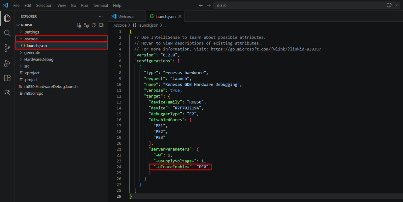
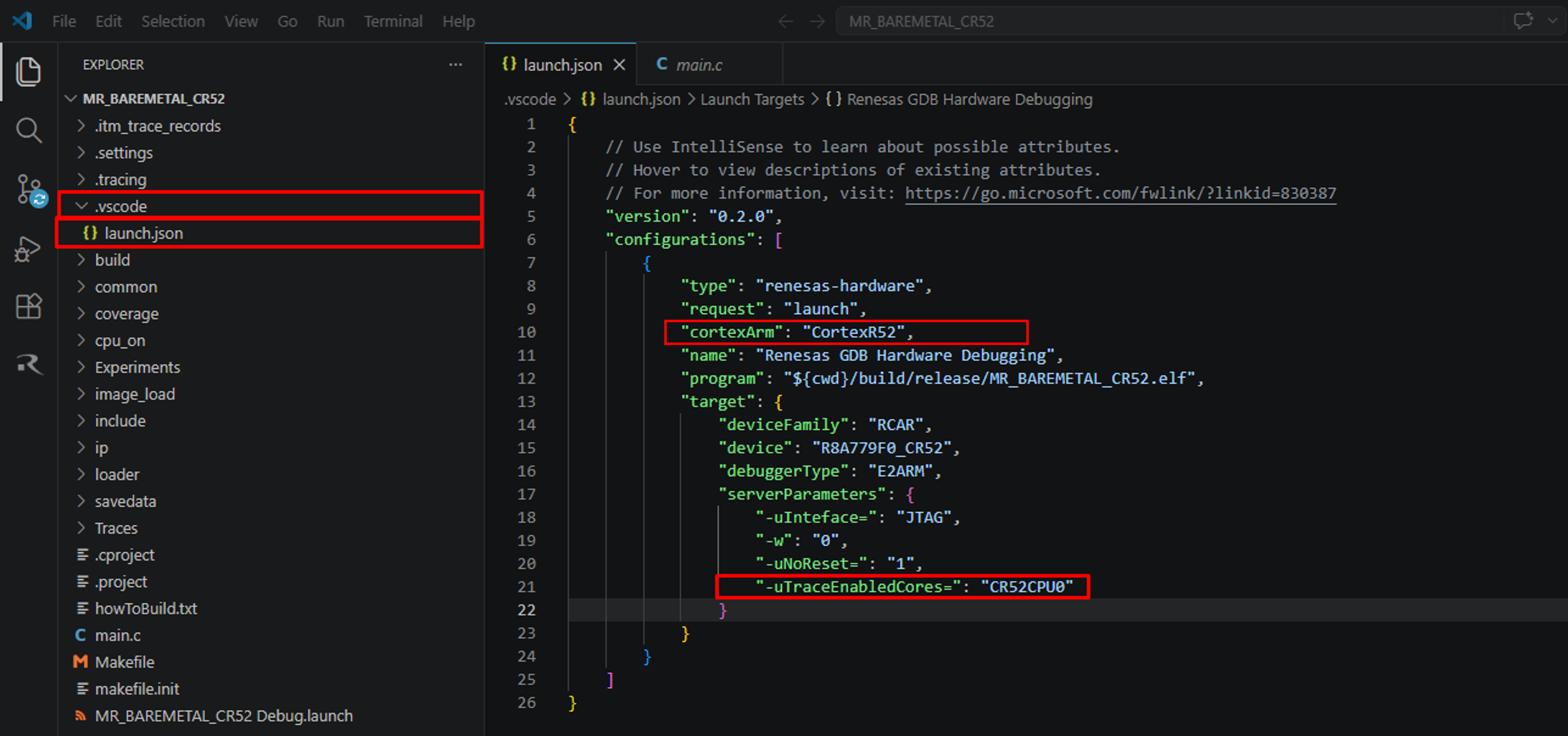
To use the Profile view, the user must enable trace data in the launch.json file. Follow these steps:

Step 1: Open the debug project.

Step 2: Navigate to Explorer > .vscode > launch.json

Step 3: Add the appropriate trace option:

• For RH850 devices, add argument “-uTraceEnable =” : “Core Name”

• For R-Car devices, add argument “-uTraceEnableCores =” : “Core Name” and “cortexArm”: “<Cortex_Name>”

10.4. Operate the Profile view

This section introduces how to operate the Profile view.

To view function profiling results, open the Profile view before running the program. Once the program is suspended, profiling information for all executed functions is displayed. The profiling data provides details such as execution time and invocation count for each function, enabling performance analysis and optimization.

10.4.1. Open Profile view

Follow the steps below to open the Profile view during debugging:

Step 1: Start debugging the program

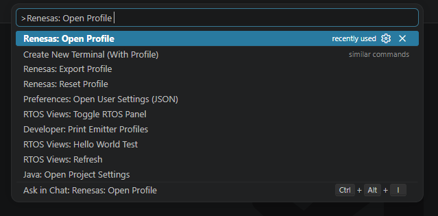
Step 2: Press F1 to open the Command Palette

Step 3: Select “Renesas: Open Profile” from the Command Palette

10.4.2. Collect and analyse the data in the Profile view

This chapter describes how to collect data in the Profile view.

To collect the profile data, follow these steps:

Step 1: Click the Continue button to run the program.

Step 2: Wait until the program suspends at a breakpoint if one has been set previously, or click the Pause button to stop program execution.

Note

For multi-session debugging, each session must be started individually before running all sessions together. To run all sessions simultaneously, select the launch session and click Resume All to run the program. Click Suspend All to stop program execution.

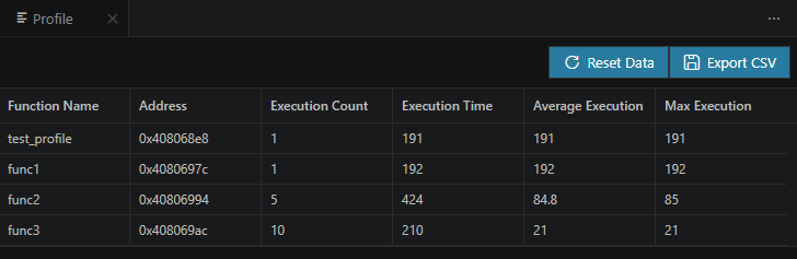
Each row in the Profile table represents a function. The Profile view displays the following information for each function:

• Function Name: The name of the executed function.

• Address: The start address of the function.

• Execution Count: The number of times the function has been executed.

• Execution Time: The amount of time spent in the function (unit is execution cycle).

• Average Execution: The average amount of time spent in the function (Execution Time/Execution Count).

• Max Execution: The maximum execution time recorded for the function.

10.4.3. Reset Profile Data

This section describes how to reset the values in the Profile view without restarting the debug session. This feature clears accumulated profiling data from previous runs, enabling more accurate performance analysis of a specific code segment or function.

Step 1: Collect data by running the program

Step 2: Click the Reset button to clear the profiling data.

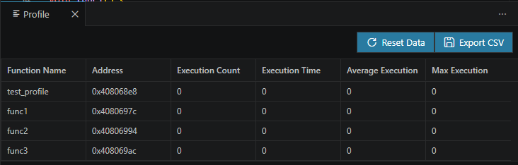
When the Reset button is clicked, the Function Name and Address values are retained, while Execution Count, Execution Time, Average Execution, and Max Execution are reset to 0. If any execution-related field currently displays “-”, it remains unchanged and continues to display “-” instead of being reset to 0.

10.4.4. Export Profile Data

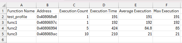
This section describes how to export data from the Profile view. The export feature allows profiling data to be saved as a CSV file for later analysis, sharing, and offline review.

To export the data, follow these steps:

Step 1: After data collection is complete, click Export to CSV.

Step 2: Select the destination folder and enter a file name.

Step 3: Click Export.

The exported CSV file contains the same information displayed in the Profile view.

10.5. Limitations

10.5.1. The display of Execution Time

The Profile view displays execution time only on devices that support trace timestamps.

Because execution time is derived from trace data, the unit of the displayed value depends on the trace timestamp specification of the target device. Execution time may be inaccurate if branch information is missing or lost in the trace data. In addition, no profiling information is displayed for functions that are not included in the trace data.

Execution time is calculated only for functions that have returned. If program execution stops while a function is still running, the execution time for that function may not be reflected in the results.

10.5.2. Effects of Trace Capacity on Data Collection

Profile results are collected based on the available trace capacity. If the Trace plugin is disabled, the maximum trace capacity supported by the Trace plugin is used. If the Trace plugin is enabled, the currently configured trace capacity is used.

A larger trace capacity allows more profiling data to be collected, but it also increases the time required to generate the profile results. If the trace capacity is too small, information about executed functions may be incomplete or inaccurate.